
When developing a real-time architecture, there are two fundamental questions that you need to ask yourself in order to make the right technology choice:
-
Freshness – how fast does the data need to be available?
-
Query latency – how fast do you need to be able to retrieve the data once it is available?
For the past ten years, Bigtable has served as critical infrastructure to support both of these questions for large-scale, low-latency use cases such as fraud detection, data mesh, recommendation engines, clickstream, ads serving, internet-of-things insights, and a variety of other scenarios where having access to current data is essential for operational workflows.
At the same time, increased demand for AI and real-time data integration in today’s applications has thrust data analytics platforms like BigQuery into the heart of operational systems, blurring the traditional boundaries between databases and analytics. Customers tell us that they love BigQuery for easily integrating multiple data sources, enhancing their data with AI and ML, and even using data science tools such as Pandas to directly manipulate data in the warehouse. However, they also tell us that they still need to make pre-processed data in BigQuery available for fast retrieval in an operational system that can handle large-scale datasets with millisecond query performance.
To address this need, the EXPORT DATA to Bigtable (reverse ETL) function is now generally available, helping bridge the gap between analytics and operational systems, while providing the query latency that real-time systems need. Now, anyone that can write SQL can easily transform their BigQuery analysis into Bigtable’s highly performant data model and retrieve it with single-digit millisecond latency, high QPS, and replicate it throughout the world so it can be closer to users. You can also query the Bigtable data using the same SQL dialect that BigQuery uses, in preview.
In this blog, we explain three use cases and architectures that can benefit from automated on-demand data exports from BigQuery to Bigtable:
-
Real-time application serving
-
Enriched streaming data for ML
-
Backloading data sketches to build real-time metrics that rely on big data
1. Real-time application serving
Bigtable complements existing BigQuery features for building real-time applications. BigQuery’s storage format is optimized for OLAP (analytics) queries such as counting and aggregations. If your real-time application requires this type of ad-hoc analysis, BigQuery BI Engine can accelerate common queries by intelligently caching your most frequently used data. Additionally, if you need to identify a specific row (or rows) that is not based on keys but requires text filtering, including JSON, BigQuery search indexes can address these text lookups.
While BigQuery is a versatile analytics platform, it is not optimized for the real-time application serving that Bigtable is designed to deliver. OLAP-based storage isn’t always ideal for quickly accessing multiple columns within a specific row or range of rows. This is where Bigtable’s data storage model shines, making it well-suited for powering operational applications.

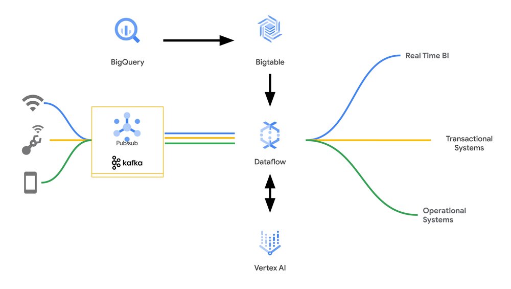
The above diagram highlights how real-time features across BigQuery and Bigtable can unite to deliver a full real-time application.
Consider using Bigtable as a serving layer when your application requires one or more of the following:
-
Single-digit millisecond latency on row lookups with consistent and predictable response times
-
Very high queries per second (QPS scales linearly with number of nodes)
-
Low-latency writes in the application
-
Global deployments (automatically replicating the data near the users)
An example
Picture this: You’re standing in the Metropolitan Museum of Art, surrounded by magnificent Greek and Roman sculptures. Who is that a statue of, and what are they doing? You pull out your phone, open the museum’s app, and point it at the statue. Instantly, a wealth of information appears on your screen — not just dry facts, but a vivid narrative that brings the artwork to life.
That’s the experience we’re crafting. But behind the scenes, delivering it is a huge technical challenge: BigQuery, our data warehouse, holds all the structured details about the artwork. However, the museum goer doesn’t want to stand around for a long time while the system queries and returns the data. Plus, we want to provide engaging text descriptions, even though our analytics platform is geared towards structured data.
Here’s where reverse ETL and Bigtable come in. Reverse ETL allows you to seamlessly move data from warehouse tables to a real-time architecture, reducing query latency. Let’s break down how to create this immersive museum app. Please note that Reverse ETL does require either a BigQuery Enterprise or Enterprise Plus edition.
Step 1: Create a Bigtable instance and serving table
If you are not familiar with Bigtable, it might be worth a quick glance at this page to understand the concepts of instances, clusters, and nodes.
The first thing you need to do is follow the instructions to create a Bigtable instance, which is a container for your Bigtable data. When you create this instance, you will need to choose the storage type of either SSD or HDD. Generally, SSD is much more performant and the right choice for production environments, but HDD can help keep costs down if you are just looking to educate yourself on how Bigtable works. While creating an instance, you also create your first cluster within the instance. This cluster needs to be in the same region as the BigQuery dataset from which you intended to load the data. However, you do have the flexibility to add clusters in other regions, which automatically receive a copy of the data from the cluster that BigQuery uses for writing data.
Once your Bigtable instance and cluster is ready to go, it’s time to create your Bigtable table, which is used as the BigQuery sink in the reverse ETL process. From the console, choose Tables in the left navigation panel and then choose Create Table from the top of the Tables screen.
In the Create a Table screen, the only thing you need to do is name the Table ID BQ_SINK and click create. We let the BigQuery Reverse ETL process create the necessary column families for us in the third step.
Alternatively, you can also use the CLI to connect to your instance and run the command cbt createtable BQ-SINK.
Step 2: Create an application profile for the BigQuery Reverse ETL job
Bigtable uses app profiles to control how an instance handles incoming requests. It’s a good practice to isolate your BigQuery data export process within its own app profile. Enable single-cluster routing within this profile to ensure your data lands in the same region as your BigQuery dataset. Additionally, set it to low priority to prevent disruptions to your primary Bigtable application traffic.
Here’s a gcloud command to create a Bigtable App Profile with these settings:
- code_block
- <ListValue: [StructValue([('code', 'gcloud bigtable app-profiles create BQ_APP_PROFILE rn –project=[PROJECT_ID] rn –instance=[INSTANCE_ID]rn –description="Profile for BigQuery Reverse ETL" rn –route-to=[CLUSTER_IN_SAME_REGION_AS_BQ_DATASET] rn –transactional-writes rn –priority=PRIORITY_LOW'), ('language', ''), ('caption', <wagtail.rich_text.RichText object at 0x3eba2ffea1f0>)])]>
Once you run this command, you should be able to see it in the Application profiles section of your Bigtable instance.

Step 3: Export the data needed for the application using SQL
Now, let’s dive into the BigQuery analysis and shape the results into a format that our artwork application can use. We’ll be working with the the_met.objects table from BigQuery public datasets. This table houses a wealth of structured metadata about each piece of art at the Met. Our goal is to generate two key elements for our art application:
-
Artist profile: A concise, structured object encapsulating information about the artist, enabling quick and efficient retrieval within our application.
-
Gen AI artwork description: A richer, narrative description of the artwork, crafted by Gemini, leveraging the metadata in the table and that is grounded by Google Search for added depth and context.
Gemini in BigQuery setup
If this is your first time using Gemini with BigQuery, you’ll need to set up the integration. Start by creating a CONNECTION to Vertex AI by following these instructions. Then, associate a model object in your dataset with the remote Vertex connection using the following BigQuery statement:
- code_block
- <ListValue: [StructValue([('code', "CREATE MODEL `[DATASET].model_cloud_ai_gemini_pro`rnREMOTE WITH CONNECTION `us.bqml_llm_connection`rnOPTIONS(endpoint = 'gemini-pro');"), ('language', ''), ('caption', <wagtail.rich_text.RichText object at 0x3eba2ffea910>)])]>
Exporting results to Bigtable
So far, everything in this tutorial has been one-time setup and configuration. We are now ready to start using data export to generate serving tables in Bigtable!
The below query provides an example but can be modified to essentially any SQL query you can create in BigQuery. You do not necessarily have to repeat all of the above steps for each new query/table.
- code_block
- <ListValue: [StructValue([('code', 'EXPORT DATA OPTIONSrn(rnuri="https://bigtable.googleapis.com/projects/[PROJECT-ID]/instances/[INSTANCE]/appProfiles/BQ_APP_PROFILE/tables/BQ_SINK",rnformat="CLOUD_BIGTABLE",rnoverwrite=true,rnauto_create_column_families=truern)rnASrnSELECTrn #use the object number as a rowkey and current time to track the changes to Bigtablern object_number as rowkey,rn CURRENT_TIMESTAMP() as _CHANGE_TIMESTAMP,rnrnrn #use Gemini to create a description of the artwork and keep the prompt used in Bigtablern STRUCT(ml_generate_text_llm_result,prompt) as generated_description,rn #create a profile of information about the artistrn STRUCT(rn `artist_alpha_sort`,rn `artist_begin_date`,rn `artist_display_bio`,rn `artist_display_name`,rn `artist_end_date`,rn `artist_nationality`,rn `artist_prefix`,rn `artist_role`,rn `artist_suffix`) as artist_infornFROMrnML.GENERATE_TEXTrn(rn MODEL [DATASET].model_cloud_ai_gemini_pro,rn (rn SELECT object_number,rn CONCAT("Describe the art object of ", object_name, " with the title ", title, " from the artist ", artist_display_name) AS prompt, rn `artist_alpha_sort`,rn `artist_begin_date`,rn `artist_display_bio`,rn `artist_display_name`,rn `artist_end_date`,rn `artist_nationality`,rn `artist_prefix`,rn `artist_role`,rn `artist_suffix`rn FROM `bigquery-public-data.the_met.objects`rn where department = 'Greek and Roman Art' LIMIT 1000rn),rn STRUCT(rn TRUE AS flatten_json_output,rn TRUE AS ground_with_google_search,rn 8192 as max_output_tokens)rn);'), ('language', ''), ('caption', <wagtail.rich_text.RichText object at 0x3eba2ffea070>)])]>
At first glance, the above query may seem daunting but it breaks down into three relatively simple parts.
-
Query the Met public dataset for artist information associated with Greek and Roman Art that we will use for our artist profile.
- code_block
- <ListValue: [StructValue([('code', "SELECT object_number, rn `artist_alpha_sort`,rn `artist_begin_date`,rn `artist_display_bio`,rn `artist_display_name`,rn `artist_end_date`,rn `artist_nationality`,rn `artist_prefix`,rn `artist_role`,rn `artist_suffix`rn FROM `bigquery-public-data.the_met.objects`rn where department = 'Greek and Roman Art' LIMIT 1000"), ('language', ''), ('caption', <wagtail.rich_text.RichText object at 0x3eba2ffea5b0>)])]>
2. Use Gemini from within BigQuery SQL to generate descriptions of the artwork based on the names of the art stored in the Met dataset and make sure it is grounded in accuracy by using Google Search.
- code_block
- <ListValue: [StructValue([('code', 'SELECT rnml_generate_text_llm_result,rnpromptrnFROMrn ML.GENERATE_TEXTrn (rn MODEL [DATASET].model_cloud_ai_gemini_pro,rn (rn SELECT object_number,rn CONCAT(rn t"Describe the art object of ", rn tobject_name, rn t" with the title ", rn ttitle, rn t" from the artist ", rn artist_display_namern ) AS promptrn FROM `bigquery-public-data.the_met.objects`rn where department = 'Greek and Roman Art' LIMIT 1000rn),rn STRUCTrn (rn TRUE AS flatten_json_output,rn TRUE AS ground_with_google_search,rn 8192 as max_output_tokensrn )rn);'), ('language', ''), ('caption', <wagtail.rich_text.RichText object at 0x3eba2ffea880>)])]>
3. Reverse ETL the result to Bigtable using the EXPORT DATA function. The options shown here overwrite the existing table, meaning it appends new rows to our Bigtable table and updates existing rows with new values when a key is already found to exist.
The key that drives our key/value lookups is based on the artwork’s object_number and we track this history of changes based on the timestamp that the query runs.
This sample automatically generates our column families, or groups of columns if the BigQuery SQL query requires it.
- code_block
- <ListValue: [StructValue([('code', 'EXPORT DATA OPTIONSrn(rnuri="https://bigtable.googleapis.com/projects/[PROJECT-ID]/instances/[INSTANCE]/appProfiles/BQ_APP_PROFILE/tables/BQ_SINK",rnformat="CLOUD_BIGTABLE",rnoverwrite=true,rnauto_create_column_families=truern)rnASrnSELECTrn#use the object number as a rowkey and current time to track the changes to Bigtablern object_number as rowkey,rn CURRENT_TIMESTAMP() as _CHANGE_TIMESTAMPrn t……………'), ('language', ''), ('caption', <wagtail.rich_text.RichText object at 0x3eba2ffea850>)])]>
Now that you understand how to do these tasks, you can return to the first query to see how it all comes together. To transform the BigQuery analysis into a Bigtable serving table, simply run that SQL query.
Step 4: Query the low latency serving table from Bigtable using GoogleSQL
Our pre-processed artwork data is ready to be used by our mobile application. Jumping over to the Bigtable console, on the left-hand navigation, choose Bigtable Studio and then Editor. Now, you can test your low-latency serving query for your application with the following SQL.
- code_block
- <ListValue: [StructValue([('code', "select _key, artist_info, rngenerated_description['ml_generate_text_llm_result'] as generated_descriptionrnfrom BQ_SINK"), ('language', ''), ('caption', <wagtail.rich_text.RichText object at 0x3eba2ffeae20>)])]>

This Bigtable SQL statement returns an artist profile as a single object as well as a generated text description column, which is exactly the data needed for your application. This serving table can be integrated with your application using any of Bigtable client libraries, including C++, C#, Go, Java, HBase, Node.js, PHP, Python, and Ruby.
2. Enriching streaming data for ML with Dataflow and Bigtable
A second popular use case for Reverse ETL between BigQuery and Bigtable is to take historical information such as customer purchase history in Bigtable, and use it as an input for ML inference models. The historic data stored in BigQuery provides a wealth of information that you can use as features for models for a variety of use cases, from recommendation systems to fraud detection. For example, knowing the contents of a customer’s shopping cart, or whether they browsed similar items before, can bring valuable context to clickstream data that feeds into a recommendation model. Identifying a fraudulent in-store credit card transaction requires much more information than what’s in the current transaction — for example, the location of the prior purchase, count of recent transactions or whether a travel notice is in place. By bringing this data to Bigtable, you can easily enrich event data being streamed via Kafka or PubSub with historical data, at high throughput and in real-time.
To do this, you can use Dataflow along with the built-in Enrichment transform for Bigtable. In fact, you can build these architectures with just a few lines of code!
- code_block
- <ListValue: [StructValue([('code', 'import apache_beam as beamrnfrom apache_beam.transforms.enrichment import Enrichmentrnfrom apache_beam.transforms.enrichment_handlers.bigtable import BigTableEnrichmentHandlerrnrnbigtable_handler = BigTableEnrichmentHandler(…)rnrnwith beam.Pipeline() as p:rn output = (prn …rn | "Create" >> beam.Create(data)rn | "Enrich with Bigtable" >> Enrichment(bigtable_handler)rn …rn )'), ('language', 'lang-py'), ('caption', <wagtail.rich_text.RichText object at 0x3eba2ffea0d0>)])]>
3. Backloading data sketches
A data sketch is a compact summary of a data aggregation that captures all the necessary information to either extract an aggregation result, continue a data aggregation, or merge it with another sketch, enabling re-aggregation. Bigtable supports data sketches with specialized conflict-free replicated data types (CRDT) that are designed to efficiently count data across a distributed system. This is crucial for real-time event stream processing, analytics, and machine learning applications.
Traditionally, managing these kinds of aggregations in distributed systems presents a challenge: prioritizing speed often sacrifices accuracy, and vice versa. Bigtable has aggregation data types that enable efficient and accurate distributed counting. These specialized column families allow each server to update its local counter independently, using mathematical properties to ensure these updates converge to the correct final value regardless of order, and eliminating the need for performance-hindering locks. Ultimately, these aggregation data types are essential for use cases such as fraud detection, personalization, and operational reporting.
These data types are also fully integrated with BigQuery’s EXPORT DATA functionality and interoperate with BigQuery Data Sketches (when the same sketch type is also available in Bigtable). This can be very useful if you want to backload your initial application with historical data or if you need to update a real-time counter with updates from an additional source outside of the streaming ingestion.
To use this functionality, you simply need to add an aggregate column family with a command and then export the appropriate data . Here’s some sample code from our museum app:
- code_block
- <ListValue: [StructValue([('code', 'EXPORT DATA OPTIONSrn(rnuri="https://bigtable.googleapis.com/projects/[PROJECT-ID]/instances/[INSTANCE]/appProfiles/BQ_APP_PROFILE/tables/BQ_SINK",rnformat="CLOUD_BIGTABLE",rnoverwrite=true,rnauto_create_column_families=falsern) ASrnSELECTrn#use the object number as a rowkey and current time to track the changes to Bigtablern met.object_number as rowkey,rn CURRENT_TIMESTAMP() as _CHANGE_TIMESTAMP,rn artist_input as data_sketchrn FROM `bigquery-public-data.the_met.objects` metrn INNER JOINrn (rn SELECTrn artist_display_name,rn HLL_COUNT.INIT(artist_display_name) as artist_inputrn FROM `bigquery-public-data.the_met.objects`rn where department = 'Greek and Roman Art'rn GROUP BY artist_display_namern ) ARTIST_COUNTrn on ARTIST_COUNT.artist_display_name = met.artist_display_name'), ('language', ''), ('caption', <wagtail.rich_text.RichText object at 0x3eba2ffea2b0>)])]>
On the Bigtable side, you can then add to this batch update with real-time updates and then call the HLL_COUNT.EXTRACT SQL function on the data sketch to produce an estimated count of artists that includes the historical information from BigQuery.
What’s next
Support for Reverse ETL between BigQuery and Bigtable goes a long way towards addressing query latency in real-time systems, but there’s plenty more to do! With continuous queries, we are hard at work on the data freshness component of real-time architectures. Currently in preview, continuous queries let you continuously replicate new data from BigQuery as it arrives into Bigtable and other sources. You can even use it with Python transformations in BigFrames through a StreamingDataFrame, ready for testing now.
To get started with Reverse ETL for on-demand data exports that address query latency and is now GA, learn more in the documentation.